Introduction
I recently took the excellent course on Machine Learning with Python from MIT. In one of the forums somebody asked about how to perform calculations of the expectation maximization (EM) algorithm without for loops. I wrote an answer about how broadcasting can be implemented in numpy to perform vectorized operations that simplify and speed up execution of the code. Because of the relevance of the topic and response from my fellow classmates, I have decided to extend the explanation and share it in this post. First I’ll show how broadcasting works with arrays of different dimensions, and then I’ll use it to implement the K-means clustering algorithm. My goal is to show in a visual way how broadcasting works, hoping it will help anybody struggling with the concept.
Broadcasting
Broadcasting can help us avoid using for-loops in arithmetic operations with vectors, matrices and multidimentional arrays. I initially learned about it in this great article on array programming with numpy; but, it took me some time to figure out how to know which dimensions to expand in a matrix in order to make broadcasting work. I found it difficult to visualize what a matrix would look like after an operation reduced one of its dimensions. This all became clear once I understood how numpy orders the dimensions of a matrix; after that it just became a matter of reshaping matrices and keeping track of their dimensions during broadcasting operations. Before I dive into those concepts, I’ll show you a few examples to help us build a simple understanding of broadcasting.
Vector-Scalar Example
The simplest example I can think of is the subtraction of a scalar from a vector. This operation is commonly used to center, or shift, a vector with respect to a given value. Let’s say we have the vector \(x\) of a given dimension \(d\) and want to subtract the value \(1\) from each element. Assuming we have the values of \(x\) in the numpy array x, we can use a for-loop and do:
y = x.copy()
for i in range(len(x)):
  y[i] = x[i] - 1
or, we can do:
y = x - 1The last piece of code is shorter and more intuitive since that’s how we also write that operation in paper; but how does numpy know how to subtract 1 from each element in x? That’s where broadcasting comes in; the image below shows how it happens in this case,
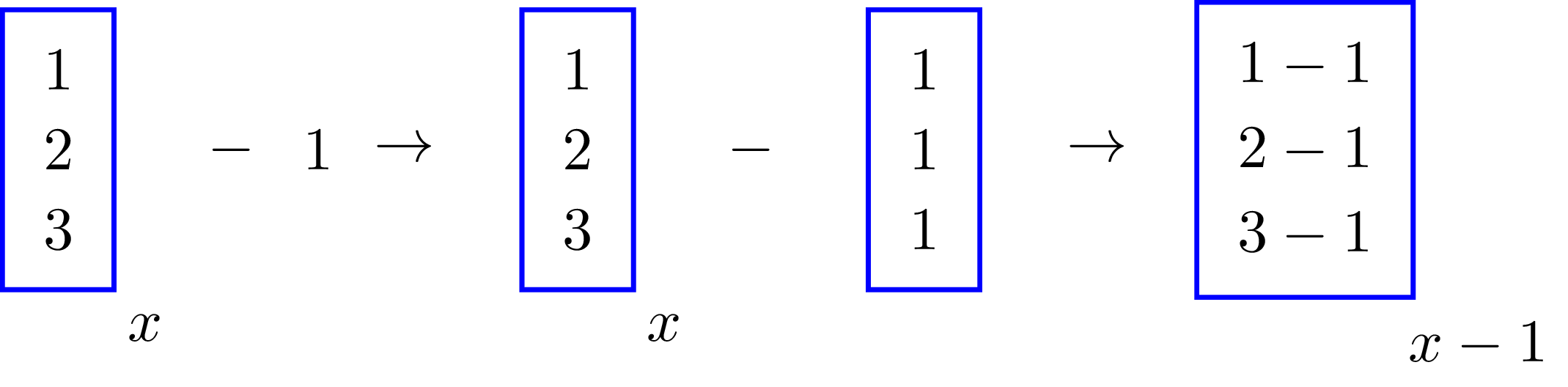
The value \(1\) was repeated, or broadcasted, along the longest dimension of \(x\) and then subtracted from each element of \(x\). Broadcasting happened this way because of the shapes, or dimensions, of \(1\) and \(x\); had their shapes been different, we would’ve had to manipulate these in order to perform the subtraction. In fact, the trick to understand broadcasting lays upon understanding the shapes of the terms we’re dealing with, and how to modify them.
Matrix-Vector Example
Let’s now increase the dimension of the objects and subtract a vector \(\mu\) from a matrix \(X\) and call the difference \(dX\); this operation is equivalent to centering the data in a matrix around a point. Each row of \(X\) is composed of a d-dimensional vector \(x_i\), and the centering vector \(\mu\) shares the same dimension of \(x_i\). In matrix notation, the data set is
\[ X = \left[\begin{array}{c}x_1^T\\ x_2^T \\ \vdots \\ x_n^T \end{array}\right] \]
and it’s centered as
\[ dX = X - 1_{n} \mu^T = \left[\begin{array}{c}x_1^T - \mu^T\\ x_2^T - \mu^T \\ \vdots \\ x_n^T - \mu^T \end{array} \right] \]
The term \(1_{n}\) is a vector with \(n\) values of \(1\). Now, assuming that we have numpy arrays with the matrix X and vector mu, we obtain the centered matrix dX with the line
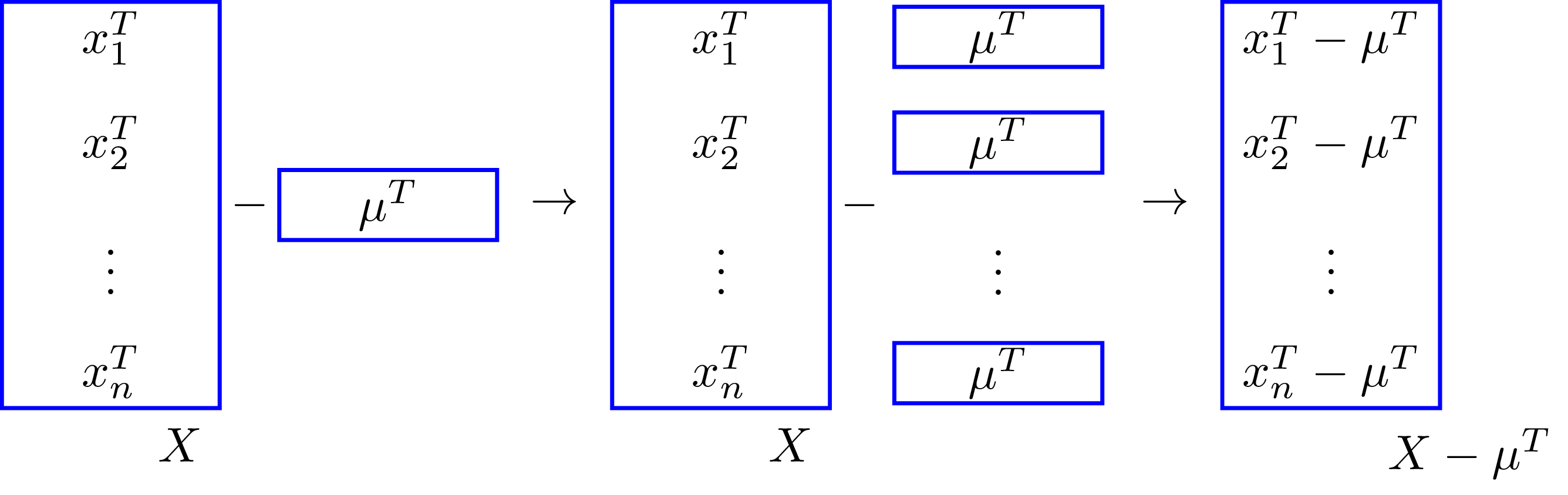
dX = X - muThe way the code is written is very similar to how we wrote the operation in the equation above; this similarity is one of the beautiful and powerful features of numpy broadcasting. The above computation happens assuming that the shape of X is \((n, d)\), and mu is a 1D array of shape \((d, )\), or a 2D array of shape \((1, d)\). Why can we use a 1D or 2D array for mu? This is because in numpy 1D arrays are considered row vectors when using them in operations with higher dimensional arrays. Furthermore, the rightmost value of the shape of an array corresponds to the number of columns of the array. In this case the matrix \(X\) and vector \(\mu\) match the number of elements \(d\) in the column dimension. Broadcasting repeats the vector \(\mu\) \(n\) times along the row-dimension. Here’s a sketch of that:
Matrix-Matrix Example
Now, let’s say you want to center the matrix \(X\) around \(m\) different vectors \(\mu_j\) contained in a matrix \(M\) that looks like this
\[ M = \left[\begin{array}{c}\mu_1^T\\ \mu_2^T \\ \vdots \\ \mu_m^T \end{array} \right] \]
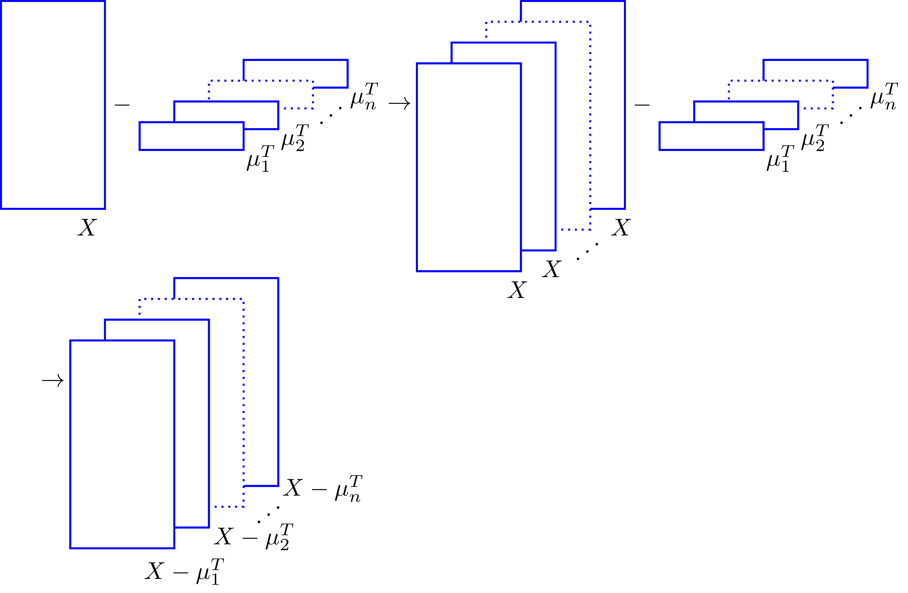
This type of centering comes up in algorithms like K-Means clustering or Expectation-Maximization. In this case we can use broadcasting by arranging \(M\) in such a way that \(X\) is repeated along a dimension of \(M\) from which \(\mu_j\) is subtracted. We can visualize this in the following sketch,
Now, how do we arrange the shape of \(M\) in the form shown above? That’s where array shapes and reshaping come into play.
Array Shapes
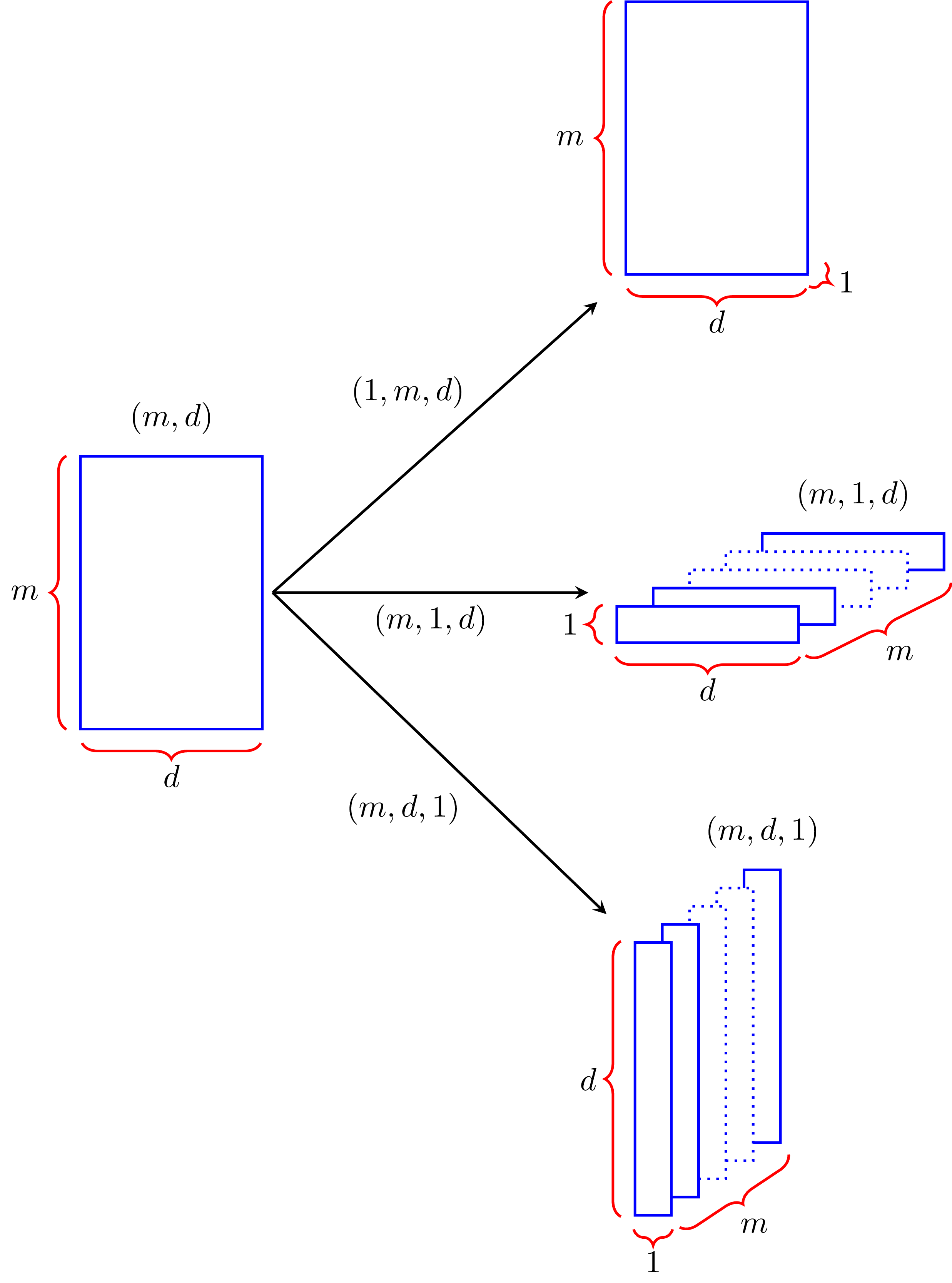
I already mentioned that the first number on the right of an array shape corresponds to the number of columns in the array; now, the second number from the right corresponds to the rows of the array, and the third number corresponds to its number of layers. If we consider \(M\) to be in a 3-dimensional space, counting from the right, the first number corresponds to the x-axis, the second to the y-axis and the third to the z-axis. Knowing this, we can add extra dimensions to \(M\) to shape it in a way that’s useful for us. If its shape is \((m, d)\), it means that we have \(m\) rows and \(d\) columns, but if we add another dimension and make the shape \((m, 1, d)\), we now have \(m\) layers, \(1\) row and \(d\) columns; similarly, a shape of \((m, d, 1)\) provides us with \(m\) layers, \(d\) rows and \(1\) column. These shape transformations look like this:
You increase the dimension of an array by slicing with np.newaxis or None in the position of the dimension you want to add. Assuming that M is a numpy array with shape \((m, d)\), you obtain the shapes
- \((1, m, d)\) with:
M[None, :, :] - \((m, 1, d)\) with:
M[:, None, :] - \((m, d, 1)\) with:
M[:, :, None]
Broadcasting in multiple dimensions
From the figure above, the second item in the previous list corresponds to the reshaped version of M we need. Thus, the broadcasted version of \(X - \mu_j\) would be computed as
dX = X - M[:, None, :]In this operation, numpy expands the shape of X to \((1, n, d)\), and broadcasts its values \(m\) times along the first dimension producing an \((m, n, d)\) array; then it repeats \(n\) times the reshaped version of M (with shape \((m, 1, d)\)) along its second dimension, producing another \((m, n, d)\) array; finally, it performs element-wise subtraction to create the array dX with shape \((m, n, d)\).
If we are interested in the distance between each point \(x_i\) and vector \(\mu_j\) we just calculate the 2-norm of the array dX along its column dimension; we do this because the difference \(x_i - \mu_j\) is stored in each row of dX, and we’d have to move across its columns in order to sum the squared values of the elements of \(x_i - \mu_j\). The code that does this is:
distance = np.linalg.norm(dX, axis=2)We didn’t specify the 2-norm in the previous function, because this norm is a default parameter. For a different norm, we would have to include the parameter ord; for example, ord=1 or ord=inf.
Since we calculated the norm across the column dimension of dX, this dimension will vanish and the new array will keep the shape of the remaining dimensions, this is \((m, n)\); therefore, the array distance will have \(m\) rows and \(n\) columns. The resulting distance between the vectors \(x_i\) and \(\mu_j\) is stored in the ijth position of the distance array.
K-Means Clustering Example
Let’s implement the k-means clustering algorithm using broadcasting. K-means clustering partitions a data set into \(k\) sets and assigns each sample of the set to the cluster with the nearest center, or mean value.
The first step in the algorithm is to decide how many clusters we’ll use to gather the data; after that, we initialize the algorithm with cluster centers randomly selected from points of the data set. At each iteration of the algorithm we calculate the distance of each point to the centers and assign the points to the cluster with the nearest center. We calculate new centers for these clusters and replace the old centers. We stop the iterations after the norm of the difference between the new and old cluster centers fall below a given threshold.
An implementation of the K-means clustering algorithm is shown below. The first 4 lines of code are used to set the seed of the random number generator and build the data set; we will generate data around 3 points, and will select the number of clusters \(k\) to be 3, although we could use any value for \(k\).
The only for-loop in the algorithm is used to assign the points to their nearest clusters and update the center of these clusters. The rest of the code is just array operations to center the data, calculate the distance of the data points to the cluster centers, and finding the nearest center to each point. I wrote the shape resulting after each operation at the end of each line in order to keep track of the shapes, and keep a mental image of how the arrays are changing.
import numpy as np
# Create data set of 15 random samples around (-3, 3), (0, 0), (3, 3)
np.random.seed(1)
points = np.array([[-3, -3], [0, 0], [3, 3]])
X = points[:, None, :] + np.reshape(0.7071*np.random.randn(100*3*2), (3, 100, 2))
X = np.reshape(X, (300, 2)) # Shape: (300, 2)
# Select random initial set of 3 centers from the original data set
k = 3 # Number of clusters
M = X[np.random.choice(X.shape[0], k, replace=False), :] # Shape(3, 2)
init_M = M.copy() # Save initial centers
# K-Mean Clustering Algorithm
center_difference = 1
while center_difference > 0.001:
dX = X - M[:, None, :] # Center matrix X around vectors in M. Shape: (3, 300, 2)
distance = np.linalg.norm(dX, axis=2) # Calculate distance between points and centers. Shape: (3, 300)
id_vals = np.argmin(distance, axis=0) # Get index value of nearest centers. Shape: (300, )
old_M = M.copy()
for i in range(M.shape[0]):
M[i, :] = np.mean(X[id_vals == i, :], axis=0) # Assign points to clusters and calculate new centers
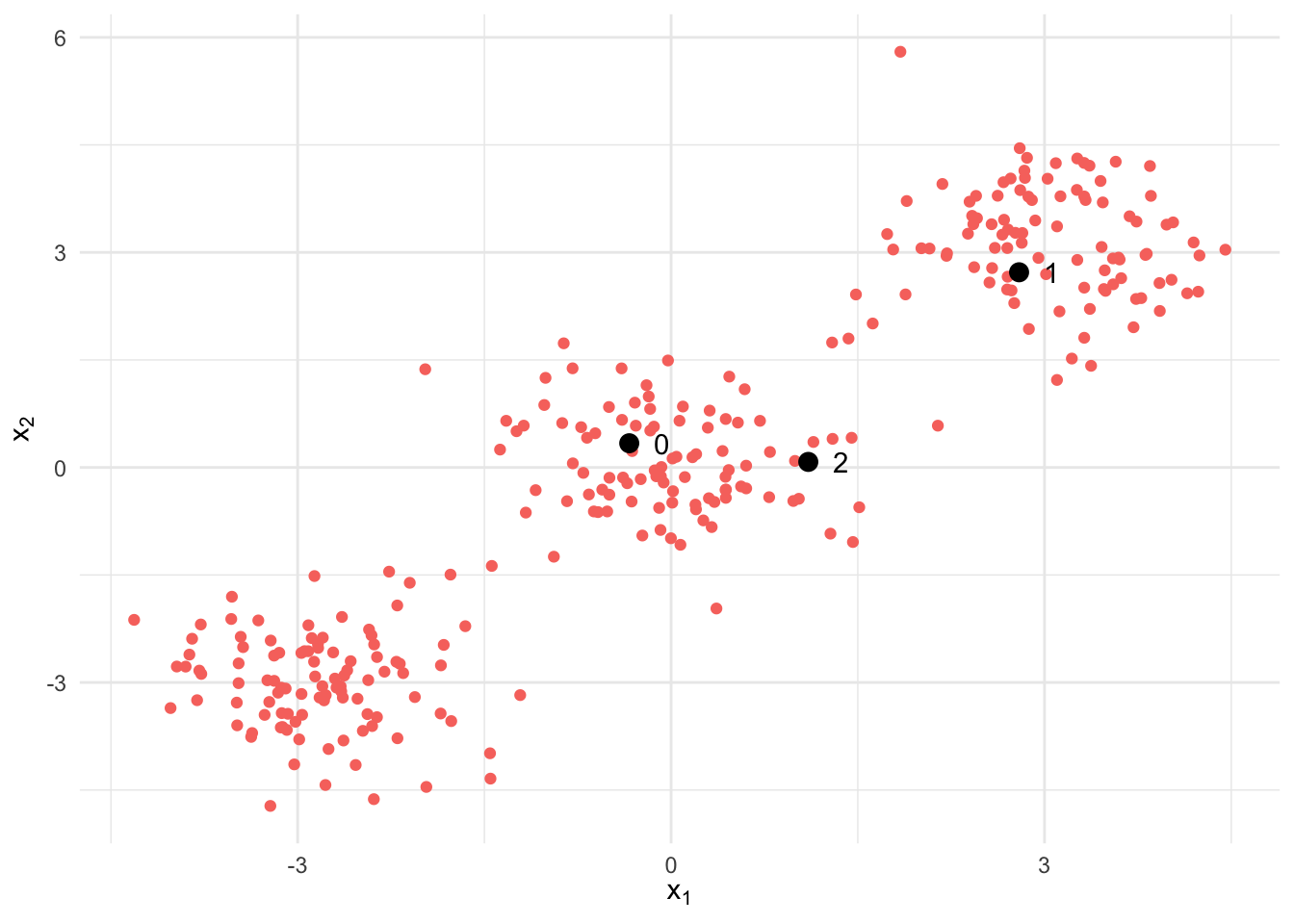
center_difference = np.linalg.norm(M - old_M) # Difference between the new and previous centersThe figure below shows the data set used to train the algorithm, as well as the points used as initial centers of the clusters. We can clearly see there are 3 clusters roughly centered around the points \((-3, -3)\), \((0, 0)\) and \((3, 3)\).
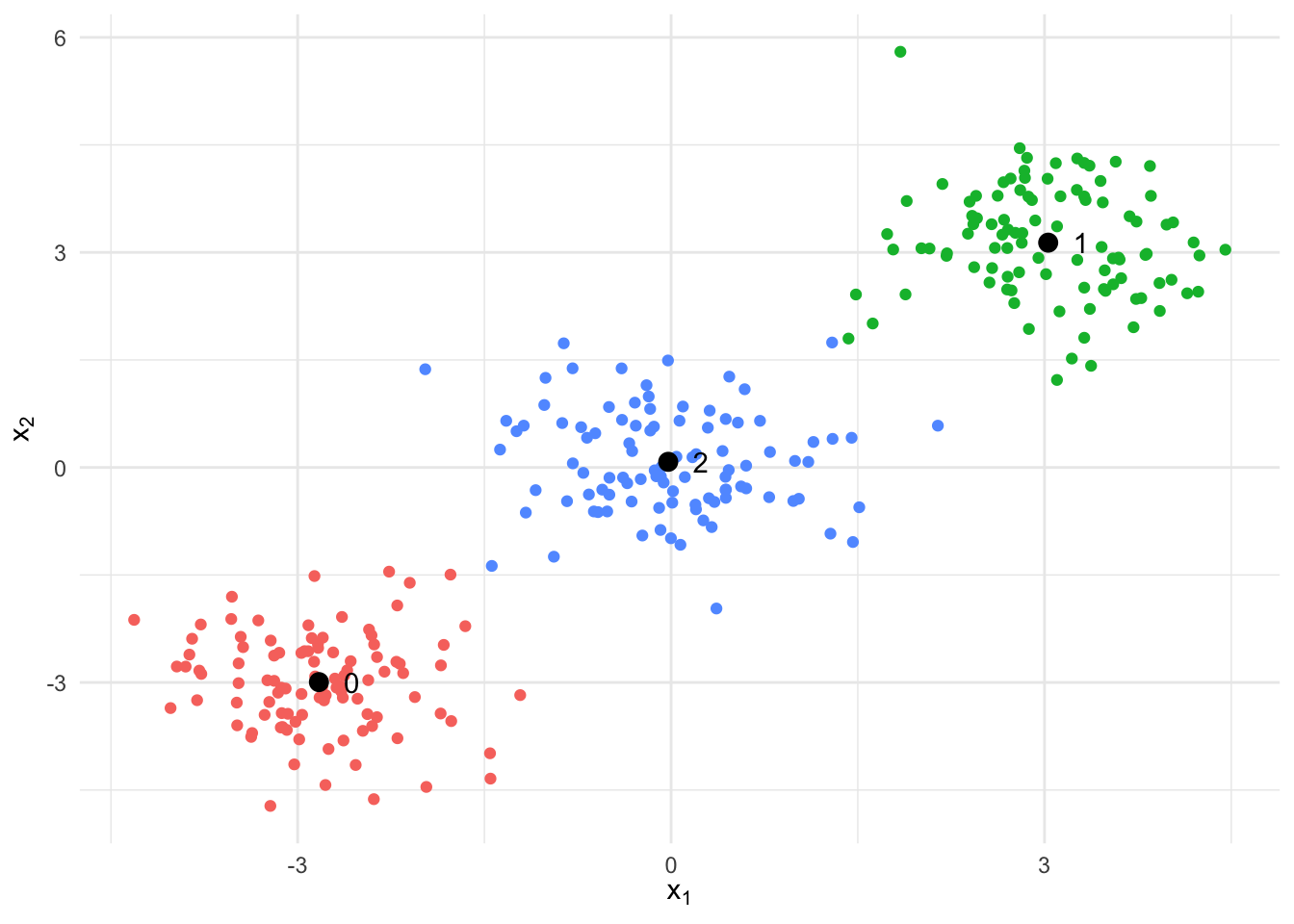
In the following plot we see the clustering results after the algorithm has converged. The resulting centers are very closed to the values we visually estimated.
Conclusion
Broadcasting is a powerful tool to simplify and expedite array computations in Python. I hope the explanation I presented here helps you understand how to reshape arrays to perform broadcasting operations. My final advice is that you try to visualize what’s going on whenever possible, and keep track of the shapes you’re obtaining; doing that will make broadcasting much easier for you. Happy coding and thank you for reading!